Think of a skater.
Pulling the arms inward can increase rotation. In a fluid, inward transport can also strengthen a vortex, while viscosity redistributes momentum.
Meet the forces inside a swirl. Move through time and watch what changes.
Your browser may have WebGL disabled. The controls and numerical experiments below still work.
A schematic path through the vortex. Move the tracer to see where it travels.
Experiment 1 of 3 · Make a prediction
Viscosity smooths differences in motion. Turn it up, then press play.
Schematic paths and toy decay. Not a fluid solver.
This first view uses speed = exp(−2νt) to illustrate friction, not an exact fluid solution. The paper views use the source’s leading-core scaling laws.
All numbers are relative to the start of the illustration. Colours distinguish regions, not calibrated speeds. The paper timeline begins at a developed core and stops before t = 1.
The fast-moving region loses volume faster than its speed squared grows. Trace the curves to move through time.
Normalized time t · vertical scale is logarithmic · both start at 1×
The Navier–Stokes equations balance motion, pressure, friction and outside forces. The puzzle is whether that balance always stays smooth.
Pulling the arms inward can increase rotation. In a fluid, inward transport can also strengthen a vortex, while viscosity redistributes momentum.
Viscosity is internal friction. It smooths differences in motion between neighbouring fluid layers. The question is whether this smoothing always wins.
The paper claims a specially forced flow whose speed becomes unbounded in a shrinking region. “Blowup” is a mathematical singularity, not an explosion.
Tap a term to translate it.
Also: ∇·u = 0. Fluid does not pile up as it flows inward; it must flow out elsewhere.
This experience is based on Section 2 of Finite Time Blowup for Navier–Stokes, attributed to OpenAI in the supplied paper. It explains the claimed construction without validating its proof.
Read the source paper ↗Explore the Blender scene in Higgsfield ↗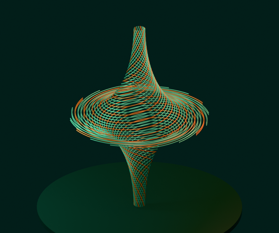
The paper views use normalized scaling laws with τ = 1 − t and h = 0.005: radius ∝ τ⁰·⁵; axial length ∝ τ⁰·⁴⁹⁵; speed ∝ τ⁻⁰·⁵⁰⁵; core volume ∝ τ¹·⁴⁹⁵; core energy ∝ τ⁰·⁴⁸⁵. Constants are set to one for illustration. These are leading-core scales, not exact whole-flow measurements.
No. The three-dimensional paths and edge pulses are schematic. We do not solve the Navier–Stokes equations, reproduce the force or residual corrections, or model the full exterior. The timeline begins with a developed core; it omits the paper’s startup from rest. The display stops at t = 0.995, before the singular time t = 1.
The paper constructs different flows for each positive viscosity. Changing viscosity while holding this scene fixed would not reproduce those constructions. The first view instead uses a separate toy decay law, speed = exp(−2νt), to illustrate friction. It is not an exact Navier–Stokes solution.
The mathematical model treats fluid as a continuous medium. A singularity concerns that idealized model; it does not show that real water reaches infinite speed. Molecular effects and other physics matter outside the model’s range.
Read the authors’ announcement and the Clay Mathematics Institute problem page. This experience makes no claim of independent verification or prize acceptance.